Stimulus

Overview

The stimulus schema is a self-contained application that generates, presents, and records visual stimuli using PsychToolbox.

Monitor Requirements

In order to view the stimulus, one needs 2 monitors at minimum while setting one of the monitors’ xscreen number higher than the other (e.g. xscreen 0 for monitor 1 and xscreen 1 for monitor 2). This process can be tricky depending on how you initially installed your monitors and set up your xscreens.

If you have a GPU on your machine, one way to check whether you have 2 xscreens is simply checking Nvidia X Server Settings

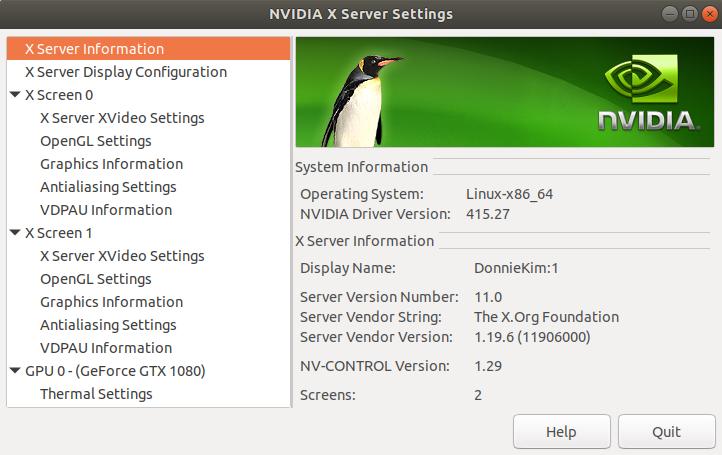
As you can see above, there are 2 x Screens set up.

It is best to consult with Chris Turner or Saumil Patel to configure xscreens.

Software Requirements

Stimulus package is written in MATLAB, thus all the packages required below must be known to MATLAB environment.

MATLAB (MUST BE R2016b or above)

• PsychToolbox : Stimulus package uses PsychToolbox as a backend

• datajoint : It is best to simply install via Add On on MATLAB console

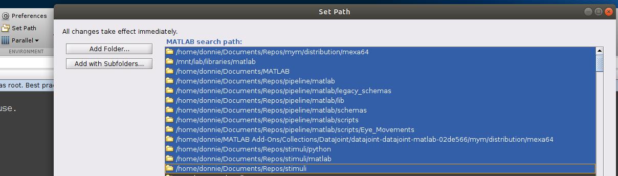
Following packages must be cloned and added to PATH of the MATLAB

• mym : datajoint extension to recognize data type BLOB

• pipeline : need to be able to access experiment module

• stimulus : stimulus package itself

In order to add these packages to PATH, click Set Path on MATLAB console and Add with Subfolders. See image below for what needs to be added

How to run existing stimulus

Unless you need to generate your own stimulus kind, you will simply run the exsiting stimulus. Here, we will demonstrate how to run manually on your computer. Note, when you actually run the experiment, you will do it through 2p master MATLAB panel. Below steps are, however, still useful when you generate your own stimulus and need to debug/troubleshoot.

Step 1: Initialize screen

stimulus.open

Step 2: Generate stimulus conditions and queue trials

Stimulus trials are generated and queued by the scripts in the +stimulus/+conf directory. You need to know which configuration script needs to be run.

For example, to prepare the singledot stimulus, execute

stimulus.conf.singledot

While the stimulus is loaded, you will see a sequence of dots . and asterisks *, which respectively indicate whether the conditions are computed anew or are loaded from the database. Some stimuli take a long time to compute and you might like to run the configuration before you begin the experiment. On subsequent runs, the computed stimuli will be loaded from the database and will not take as long.

Step 3. Run the stimulus

The stimulus must be run for a specific scan in the experiment.Scan table. Table experiment.Scan contains a dummy entry that can be used for testing. Its primary key is struct(‘animal_id’, 0, ‘session’, 0, ‘scan_idx’, 0). During the experiment, the correct scan identification must be provided.

stimulus.run(struct('animal_id', 0, 'session', 0, 'scan_idx', 0), false)

Note, false is given so that we do not log our dummy entries to stimulus.Trial() table.

Step 4. Interrupt and resume the stimulus

While the stimulus is playing, you can interrupt with Ctrl+c. The stimulus program will handle this event, cancel the ongoing trial, and clear the screen. To resume the stimulus, repeat the stimulus.run call above. Or to queue a new set of trials, run the configuration script again.

Step 5. Exit

To close the stimulus program,

stimulus.close

Stimulus Repository Structure

The structure of Stimulus repository can be confusing for new users and needs to be explained. The basic structure can be broken down as the following tree:

stimuli
├── python
└── matlab
  ├── +xtimulus
  ├── +imagenet
  ├── +netflix
  ├── conf
  |     ├── singledot.m
  |     ├── matisse.m
  |     ├── grating.m
  |     .
  |     .
  |     .
  └─── +stimulus
    ├── +conf
    |     ├── singledot.m
    |     ├── matisse.m
    |     ├── grating.m
    |     .
    |     .
    |     .
    ├── +core
    |      ├ Control.m
    |      ├ FIFO.m
    |      ├ Screen.m
    |      └ Visual.m
    ├── +utils
    |      ├ DataHash.m
    |      ├ factorize.m
    |      └ license.txt
    ├── SingleDot.m
    ├── Matisse.m
    ├── Grating.m
    .
    .
    .

We will only focus matlab folder.

Under matlab we have folders with + sign prepended. For MATLAB, + has a special meaning and it recognizes as a class folder. If you are familiar with Python, think +foldername as a module.py. Inside these +foldername, you have bunch of m files and you can think of them as class definitions in Python. If you need further help, you can refer to this MATLAB documentation.

For those who are not familiar with Python nor classes, just treat them as a special symbol for MATLAB to recognize that folder and m files underneath.

Let’s focus on +stimulus first. Inside +stimulus, we have +conf, +core, +utils, and whole bunch of m files:

• +conf : contains configuration files (singledot.m, mattise.m, etc) that specify parameters for some stimulus presentation

• +core : controls and interacts with your display and Psychtoolbox. Most likely, you won’t have to change anything here. But if you need to update something, consult with either Saumil or Dimitri

• +utils : some help functions. Not so important unless you can find a function to be called universally across different stimuli.

• m files (SingleDot.m, Matisse.m, etc): Display m files that dictate how the stimulus should be displayed.

Two important points here.

First, right underneath +stimulus, SingleDot.m file, for example, dictates how the single dot stimulus is displayed. We will define this file as a PRESENTATION file and will go through this particular file in Designing a New Stimulus section line by line.

Second point is singledot.m file underneath +stimulus/+conf/. This is a CONFIGURATION file that calls WHICH stimulus to be displayed and set PARAMETERS for that particular stimulus.

Also, as you get more familiar/advanced with stimuli package, `+core` will become more important and you should spend time understand what each file (i.e. Visual, Screen, Control) does inside that class folder.

Notice that for PRESENTATION file, we used camelCase as naming convention. For configuration file, we used lower case. Please keep these styles if you need to make new stimulus presentation and config files.

Now, you also notice that there is matlab/conf and matlab/+stimulus/+conf. The reason we have TWO conf folders (with difference of + sign) is that for testing a new stimulus, we put m files under matlab/+stimulus/+conf. But when we actually scan, the finalized m file must be copied over to conf in your 2pmaster scanning machine because 2pmaster only recognizes folders without + sign.

In short, the same config file, for example, singledot.m, should exist in both matlab/conf and matlab/+stimulus/+conf once finalized.

Designing a New Stimulus

There are two parts in designing:

1. Stimulus Presentation - HOW the stimulus is displayed on the monitor/projector (e.g. SingleDot.m)

2. Stimulus Configuration - PARAMETERS for the stimulus one designed. (e.g. singledot.m)

Often times, one doesn’t probably need to design a new stimulus presentation but simply modify the configuration file.

Here, we demonstrate a demo of designing a single dot stimulus

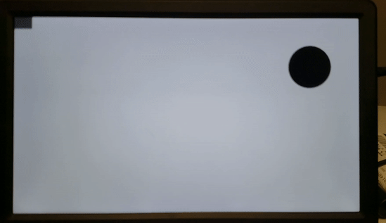
single dot stimulus demo

Stimulus Presentation

Below is the content of SingleDot.m.

%{
# single dot to map receptive field
-> stimulus.Condition
-----
bg_level                    : smallint                      # (0-255) the index of the background luminance, 0 is black
dot_level                   : smallint                      # (0-255) the index of the dot luminance, 0 is black
dot_x                       : float                         # (fraction of the x length, 0 for center, from -0.5 to 0.5) position of dot on x axis
dot_y                       : float                         # (fraction of the x length, 0 for center) position of dot on y axis
dot_xsize                   : float                         # (fraction of the x length) width of dots
dot_ysize                   : float                         # (fraction of the x length) height of dots
dot_shape                   : enum('rect','oval')           # shape of the dot
dot_time                    : float                         # (secs) time of each dot persists
%}

classdef SingleDot < dj.Manual & stimulus.core.Visual
    properties(Constant)
        version = '2'
    end

    methods
        function showTrial(self, cond)
            self.trialBacklogSize = 100;  % see stimulus.core.Visual
            Screen('FillRect', self.win, cond.bg_level, self.rect)
            width = self.rect(3);
            height = self.rect(4);
            x_pos = cond.dot_x + 0.5;
            y_pos = cond.dot_y + 0.5 * height/width;
            rect = [x_pos-cond.dot_xsize/2, y_pos-cond.dot_ysize/2, x_pos+cond.dot_xsize/2, y_pos+cond.dot_ysize/2]*width;
            command = struct('rect', 'FillRect', 'oval', 'FillOval');
            Screen(command.(cond.dot_shape), self.win, cond.dot_level, rect)
            self.flip(struct('checkDroppedFrames', false))
            WaitSecs(cond.dot_time - 1.5/self.fps);
            Screen(command.(cond.dot_shape), self.win, cond.dot_level, rect)
            self.flip(struct('checkDroppedFrames', false))
        end
    end
end

Table definition

First off, let’s start with the table defintion

single-dot-table-def

%{
# single dot to map receptive field
-> stimulus.Condition
-----
bg_level                    : smallint                      # (0-255) the index of the background luminance, 0 is black
dot_level                   : smallint                      # (0-255) the index of the dot luminance, 0 is black
dot_x                       : float                         # (fraction of the x length, 0 for center, from -0.5 to 0.5) position of dot on x axis
dot_y                       : float                         # (fraction of the x length, 0 for center) position of dot on y axis
dot_xsize                   : float                         # (fraction of the x length) width of dots
dot_ysize                   : float                         # (fraction of the x length) height of dots
dot_shape                   : enum('rect','oval')           # shape of the dot
dot_time                    : float                         # (secs) time of each dot persists
%}

If you are not familiar with datajoint MATLAB, refer to this documentation.

In this particular table, it inherits stimulus.Condition table as a primary attribute. When designing a new stimulus, you MUST have stimulus. Condition as a primary attribute.

Then, it defines bg_level, dot_level, dot_x, dot_y, etc, in secondary attributes with specific datatype with explanations. Make sure each attribute is properly explained (no generic explanation) when designing a table.

How to define a class

Now let’s look at how the class is defined and what it inherits:

classdef SingleDot < dj.Manual & stimulus.core.Visual

First, your class name must match with your filename (e.g. SingleDot). And it must inherit 2 additional classes, namely dj.Manual and stimulus.core.Visual (line 1). To inherit in MATLAB, you use “<” sign. By doing this, you declare that your table tier is Manual, and you now have access to Visual class. Every stimulus presentation file MUST inherit these two classes without any exceptions.

How to define properties

We can set some properties and one of the properties that you MUST declare is version (line 2). version is an abstract property inherited from Visual class.

As you update/modify your code in development, make sure that you version up (by whole number) as you go.

properties(Constant)
    version = '2'
end

How to define methods

We can also set methods and `showTrial` is another abstract method inherited from Visual. In other words, you MUST declare it, otherwise it will throw an error.

methods
    function showTrial(self, cond)
        self.trialBacklogSize = 100;  % see stimulus.core.Visual
        Screen('FillRect', self.win, cond.bg_level, self.rect)
        width = self.rect(3);
        height = self.rect(4);
        x_pos = cond.dot_x + 0.5;
        y_pos = cond.dot_y + 0.5 * height/width;
        rect = [x_pos-cond.dot_xsize/2, y_pos-cond.dot_ysize/2, x_pos+cond.dot_xsize/2, y_pos+cond.dot_ysize/2]*width;
        command = struct('rect', 'FillRect', 'oval', 'FillOval');
        Screen(command.(cond.dot_shape), self.win, cond.dot_level, rect)
        self.flip(struct('checkDroppedFrames', false))
        WaitSecs(cond.dot_time - 1.5/self.fps);
        Screen(command.(cond.dot_shape), self.win, cond.dot_level, rect)
        self.flip(struct('checkDroppedFrames', false))
    end
end

This particular block deserves some detailed explanation.

First, showTrial takes 2 arguments, self and cond.

self is a special keyword understood by MATLAB and MUST present as the FIRST argument when defining methods.

cond is an argument that is in struct. Inside the struct, it must have information corresponding to what is defined in table defintion such as bg_level, dot_level, etc. We will further explain how condition is generated under Stimulus Configuration.

Moving on to line 3, we have self.trialBacklogSize = 100. Now, we never defined trialBacklogSize as our property, yet it is still understood here. How? Because we inherited Visual class which has trialBacklogSize as a property! This property dictates how many trials to accumulate before logging into the trials table. If you do not specify, that is okay since the default value is set to 1.

In line 4, now we finally draw a rectangular box by calling Screen. It is advised to read this for better understanding of the explanation. Here, Screen is understood (even though we never defined what Screen is) as PsychToolbox is added in our MATLAB path. To draw a rectangular box, we specify FillRect as our first argument. Then, we must give a pointer to the window. Again, Visual class already handled it for us, and we simply call self.win. Then, we must give a color. If in black/white, it can be a scalar, otherwise in 3 elemnts long array (RGB). Lastly, we give a rect, which again can be found from Visual class. Btw, the purpose of this line is not just simply drawing a random rectangular box. It is there to specify the BACKGROUND for the dot to appear.

In line 5 and 6, we obtained width and height of our rectangle which matches the pixel dimensions of your display.

In line 7 through 9, we compute WHERE the dot should appear relative to our rectangle dimensions (here, rectangle dimension is our display dimension). Also, it also computes the size of our dot.

Line 10 and 11 are interesting. In line 10, we defined a variable “command” with 2 mappings: If rect, then its value is FillRect. If oval, then`FillOval`. In line 11, we finally make our dot. But look at the first argument, command.(cond.dot_shape). cond has dot_shape value and it can either be rect or oval according to our single-dot-table-def. Then, our first argument becomes command.rect which value is FillRect or command.oval which value is FillOval. These FillXXXX then are commands that are understood by PsychToolbox.

In line 12, we now call self.flip. To explain what this does in detail is probably out of our scope. But in short, what we have done so far upto line 11 is commanding the computer to prepare what to draw. In other words, nothing has been drawn on the display yet. In order to do so, we have to flip to fresh out frame buffer. checkedDroppoedFrames is an option to pass whether to check or not. If set true and there are more than 3 frames dropped, it will print out the dropped frame numbers.

For those interested in detail, you can click framebuffer and page flip.

In line 13, we now command to wait for cond.dot_time - 1.5/self.fps seconds. At this point, the background AND the dot are present on the display for that many seconds.

In line 14 and 15, we are repeating line 11 and 12. Why? By the time we wait n seconds from line 13, there is a chance that the n seconds we waited is off from what the screen fps is. Say our monitor shows a frame every 50 ms. But if we waited 57 ms, for example, then we are off by 7 ms and can cause a problem. To completely wipe out such discrepancy, we simply redraw and force the syncing.

Stimulus Configuration

Below is the content of singledot.m.

function singledot
control = stimulus.getControl;
control.clearAll()   % clear trial queue and cached conditions

params = struct(...
    'bg_level',    255,         ... (0-255) the index of the background luminance
    'dot_level',   0,           ... (0-255) the index of the dot luminance
    'dot_xsize',   0.125,        ... (fraction of the x length) size of dot x
    'dot_ysize',   0.125,        ... (fraction of the x length) size of dot y
    'dot_x',       linspace(-0.5,0.5,8),       ... (fraction of the x length, -0.5 to 0.5) position of dot on x axis
    'dot_y',       linspace(-0.28,0.28,5),      ... (fraction of the x length) position of dot on y axis
    'dot_shape',   'oval',       ... shape of dot, rect or oval
    'dot_time',    0.25           ... (secs) time each dot persists
    );

% generate conditions
assert(isscalar(params))
params = stimulus.utils.factorize(params);

% save conditions
hashes = control.makeConditions(stimulus.SingleDot, params);

% queue trials
nblocks = 10;
fprintf('Total time: %g s\n', nblocks*(sum([params.dot_time])))
for i=1:nblocks
    control.pushTrials(hashes(randperm(numel(hashes))))
end
end

In line 2 and 3, we first get control object and call clearAll method to clear out possible trial queues and cached conditions. It is highly recommdned to perform these two lines when designing a new stimulus.

In line 5, now we specify what we want for parameters that are defined in our single-dot-table-def.

In line 18, we then factorize our conditions. Before the factorization, condition has dox_x and dot_y values an array. By doing factorization, there exists only one value per parameter for each condition.

In line 21, now we make the conditions. Conditions is a table that contains hashes where each hash corresponds to each stimulus type for a given parameter. One can see what condition table looks like by prompting stimulus.Condition:

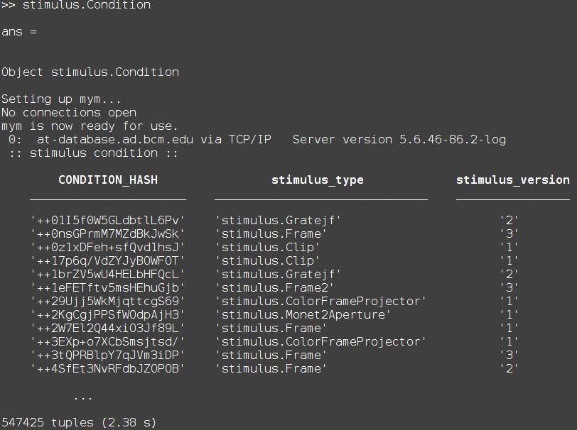
Now remember we talked about dots and astericks when we ran an existing stimulus? Those prompts are printed out from this particular line. It looks at the given stimulus type and its paramemters, and if it finds that particular combination in our stimulus.Condition table, then it simply loads that condition (with dots as loading sign). If not, then it will generate for you ( with astericks as generating sign).

From line 24 to the end dictates in WHAT sequence we want to show the conditions. Here, we call randperm to randomize the order of the conditions. Then those randomized conditions are pushed to control via control.pushTrials and displayed.

Configuration Examples

Here, we have a list of configuration with explanation. Please contribute to this page so that every stimulus we present is explained in details.

imagenet_v2

TODO Assigned to Donnie Kim

Other Resources:

GitHub: https://github.com/cajal/stimuli.git

PsychToolbox Documentation: http://psychtoolbox.org/docs/Psychtoolbox

PsychToolbox Demos: https://peterscarfe.com/ptbtutorials.html